In brief:
What I found on the internet and a few formulas I derived myself.
References to the spreadsheet I developed during my search.
Download the spreadsheet in Zip format. It can be opened in Excel, OpenOffice, LibreOffice, etc.
The fields wit formulas are protected against accidental change. The password to unprotect them is "Protect".
The lines with green text give some differences or ratios between results which should differ only slightly. If you see large numbers there then most likely there is something wrong with the formulas.
Subjects for further study
Contents:
Terminology
In the order of the spreadsheet:
Constants
Pendulum Swing Times
Foucault Precession
Intrinsic Precession
Quality factor of the pendulum
Drive timing according to the Schumacher equation
Sensitivity of the Floor Unit adjustment
Energy in the system
Forces on the cable
Forces on the mounting point
Thermal expansion of the cable
Passage times for a certain distance
Height of tip of bob at some distance from the center
Height from top for a given excursion of the cable
Dimensions and weight of a cylindrical Bob
Dimensions and parameters of the Coils
References
Articles and sites about theory and practice of several pendulums
Terminology.
In the literature about Foucault Pendulums often the following naming is used for the several parameters. I'll stick to this terminology as good as possible.
g for the accelleration of gravity on earth [9.81 m/s2] (can locally differ up to 1%, also dependent on height)
φ (fi) for the northern or southern latitude of the location of the pendulum. Southern latitude is sometimes given as negative.[degrees or radians]
L for the length of the pendulum, from the deflection point at the top to the center of mass of the bob. [m]
M for the mass of the bob.[kg] The mass of the cable is mostly neglected.
T for the period of the pendulum. [sec]
ω (omega) for the actual frequency of the pendulum. [rad/sec]
ω0 (omega-null) for the frequency at very small amplitude [rad/sec]
a for the amplitude in the desired direction, the longest axis of the ellipse. [m]
b for the amplitude of the shortest axis of the ellipse. [m]
ΩF (Omega-F) for the Foucault precession. [rad/sec]
ΩI (Omega-I) for the intrinsic precession due to the elliptical path. [rad/sec]
ΩA (Omega-A) for the siderical rotation of the earth.[rad/sec] 1 siderical rotation is approximately 23:56:4.14 [hh:mm:ss.ss]
Θ (Theta) for the angle at maximal excursion.[rad]
Q for the quality factor of the pendulum [dimensionless]
E the energy in the system systeem [Joule] (alternates beteween potential energy and kinetic energy)
In the order of the spreadsheet
Constants
The gravitational constant can be slightly different at your location.
For my location (vicinity of Arnhem, NL) I found 9.8123. source: https://upload.wikimedia.org/wikipedia/commons/c/ce/Valversnelling_in_Nederland.svg
The siderical day is defined as the rotation of the earth with respect to the far "fixed" stars. It is slightly shorter than the well known 24-hours day, because that one is related to the earth's rotation w.r.t. the sun. The earth also rotates around the sun in one year and so the difference is about 1/365 of a day.
Pendulum swing times
The exact period of a pendulum is hard to calculate because it also depends on the amplitude. Most formulas are approximations..
The most well known is:
T = 2 π √ (L/g) [sec] (1)
The theoretically exact solution with a lot of terms having a regular pattern: (2)
T = 2 π √ (L/g) * [ 1+ (1/2)2 sin2(Θ0/2) + ((1*3) / (2*4))2 sin4(Θ0/2 ) + ((1*3*5) / (2*4*6))2sin6(Θ0/2 ) + ((1*3*5*7) / (2*4*6*8))2 sin8(Θ0/2 ) + ...] [sec]
where Θ0 = arcsin (a/L)
Below is a piece of FreePascal code to calculate this formula.
Supposedly exact but converges with fewer terms which follow a (for me) unknown pattern: (3)
T = 2 π √ (L/g) * [ 1+ 1/16 Θ02 + 11 / 3072 Θ04 + 173 / 737280 Θ06 + 22931 / 1321205760 Θ08 + ...] [sec]
where Θ0 = arcsin (a/L)
An approximation which gives reasonal results without an infinite series of terms: (4)
T = 2 π √ (L/g) *[cos(θ/2)]^-{0.5*[cos(θ/2)]0.125}
The formula derived by Lima and Arun:
T = -2 π √ (L/g) * [ ln(a) / (1-a) ] [sec] where a = cos (Θ0/ 2) (5)
For the time being I use formula (2) , expanded over 3 terms.
The Foucault Precession is
ΩF = ΩA / sin φ / [1 - (3/8 * a2 / L2)] [rad/sec] For NL at 52° that gives about 31 hours for 1 rotation. (6)
For small excursions the part between [ ] can be omitted, the difference is generally a few minutes. (7)
In my calculations I use the complete form.
Intrinsic Precession of the Ellipse
Is given by
Ωe = 3/8 * ϖ0 * ab / L2 [rad/sec] (8)
where ϖ0 = 2 * π / T [rad/sec]
The Qualityfactor
The Quality factor of a resonator (also e.g. a tuning circuit in a radio receiver) is the ratio between the energy in the system and the energy loss per period.
With a Foucault pendulum it is nearly impossible to calculate the Q in advance, because the losses, mainly by air friction, are difficult to calculate.
There are however some methods to measure the Q of a practical pendulum.
1/ Measure the amplitude of the pendulum, then stop driving it and count the number of periods before the amplitude has reached half of its original value. Multiply that number by 4.53 and you have the Q.
2/ The same but count until the amplitude is 37% of the original value. Multiply by pi and you have the Q.
3/ Use both methods and take the average.
I used only method 2.
Q = π * τ / T [-] (9)
where τ is the time when the pendulum has reached 37% from the begin amplitude after stopping the drive.
Q is also defined as
Q = 2 π E / Eloss [-] (10)
where Eloss is the energy loss per period, so
Eloss = 2 π E / Q [J] (11)
and this is the energy which has to be added during each period to keep the pendulum in motion.
So per half periode half of it.
Drive timing according to the Schumacher equation
Schumacher (download) describes in his article that if the drive pulse is given on a very special moment during the swing, the precession of the ellipse (not the ellipse itself) is perfectly suppressed. It turns out that his equation [19 in the article] cannot be solved analytically, the only way is to find an optimum by iteration (trial and error)
Change "Drive Position" such that the "Ratio Left / Right" becomes 1.0 as good as possible. "Drive Position" in meter or in samples after the zero crossing then gives the optimal drive moment.
Note that Schumacher's formula is quite sensitive for the Q and for the amplitude of the pendulum. You have to know the Q and keep the amplitude under control.
As the Q is mainly determined by the air friction it will be sensitive to the viscosity of the air, which is dependent on air pressure, humidity and temperature.
Sensitivity of the Floor Unit adjustment
Based on 0.1 mm displacement per rotation of the knob.
Energy in the system
The energy in the system can be calculated in two ways. From the difference in height that the bob passes between the zero crossing and the maximal amplitude, and from the velocity of the bob at the zero crossing.
The kinetic energy at the lowest point, that is at the highest velocity, is
Ev = 1/2 M (2 π / T)2 [J] (12)
This will give a slightly incorrect result because it assumes the motion of the pendulum to be perfectly harmonic (sine shaped) and that is not the case, there are odd harmonics in the actual motion.
The height reached at the maximal excursion is:
h = L - √ (L2 - a2) [m] (13)
and so the potential energy there is:
Ep = g * M * h [J] (14)
There must be: Ev = Ep = E (15)
Forces on the cable
The maximal force appears at the center passage, there the centripetal force adds to the weight of the bob.
Fmax = M * g + M * v2 / L [N] (16)
where v the velocity at center passage, approximated by 2 * π * a / T
The minimal force appears at the end of the swing
Fmin = M * g * cos(Θ0) [N] (17)
where Θ0 the angle at maximum deviation: arcsin (L / a)
Forces on the mounting point
It may be interrresting to have a look at these figures to judge the stability of your mounting point. The slightest movement here will degrade the performance of your pendulum.
Thermal expansion of the cable
This can be important with long pendulums because it may change the height of the bob above te floorunit. This will influence the effect of the drive coil and the amplitude of the sensed signals. However, the thermal expansion of the building itself will have an influence too, but is rarely known.
Passage times for a certain distance
This is to calculate passing a certain distance in sample-ticks after the center passage.
I assumed here that the bob is making a perfect hamonic (sine-shaped) movement. That is not the case, but the deviation is a few promilles.
Height of the tip of the bob at some distance from center
The height ht of the bob-tip at a distance d from the center is:
ht = Lt *(1-cos(Θ)) where Θ = asin(dt/Lt) and Lt the length from the top to the tip of the bob.
Height from top for a given excursion of the cable
This was to calculate the height at which the magnet for the Hall Sensors had to be placed such that it makes a certain excursion.
Dimensions and weight of a cylindrical Bob
Design your own Bob.
Dimensions and parameters of the Coils
Dimensions are according to this diagram:
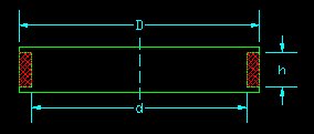
Number of wires parallel.
For the Drive Coil for the Chapel Pendulum I had available only to thin or to thick wire, and many bobines of the thin wire. So I decided to wind it with multiple wires, each to thin. This requires some extra calculation of what the final resistance would become.
Diameter of wire
I have ignored the thickness of the insulation layer.
Fill Factor.
Here it is the ratio between the total cross section of the copper wires and the available space as defined by the coil former dimensions.
If all the space is perfectly filled with round copper wire, each side-aside you may expect a fill factor of π / 4 = 0.78. In practice you will never realize that.
If the outcome is much smaller there is room for more windings. If it is larger the windings will overflow the available space.
Passage times of the Bob are given in Sample ticks after the zero passage.
You will need these values to estimate the "expect" and "missed" times in the BobControl settings.
References:
(1) can be found in any textbook about Foucault pendulums.
(2) en (3) https://en.wikipedia.org/wiki/Pendulum_(mechanics)#Arbitrary-amplitude_period
Here a FreePascal function to calculate the exact swing time.
function ExactSwingTime (Length, Amplitude, Gravity: extended): extended;
// we use the formula given in:
// https://en.wikipedia.org/wiki/Pendulum_(mechanics)#Arbitrary-amplitude_period
// as the Legendre polynomial solution
var Theta, SinHalfTheta, Term0, Term1, Term2, Term3, Term4, Term5: extended;
begin
Theta:= arcsin (Amplitude / Length); // angle at maximum position
SinHalfTheta:= sin (Theta / 2);
Term0:= 2 * pi * sqrt (Length / Gravity); // the classical approximation
Term1:= sqr (1 / 2) * power (SinHalfTheta, 2);
Term2:= sqr (3 / 8) * power (SinHalfTheta, 4);
Term3:= sqr (15 / 48) * power (SinHalfTheta, 6);
Term4:= sqr (105 / 384) * power (SinHalfTheta, 8);
Term5:= sqr (935 / 3840) * power (SinHalfTheta, 10);
ExactSwingTime:= Term0 * (1 + Term1 + Term2 + Term3 + Term4 + Term5);
// show the contribution of each term
writeln (format ('%20.18f, %20.18f, %20.18f, %20.18f, %20.18f, %20.18f',
[Term0, Term1, Term2, Term3, Term4, Term5]));
end;
(4) was found in a link which is now dead
(5) was found in Lima and Arun (download)
(6), (7) without the term between [ ] found in many publications about the Foucault pendulum.
The term between [ ] was found in Haringx and Suchtelen (download)
(8) -up are commonly known in kinematics and mechanics.
Articles and sites about theory and practice of the Foucault pendulum
The Dutch physicist Heike Kamerlingh Onnes (yes, the one from the liquid Helium and the superconductivity) had his doctoral thesis in 1879 about the Foucault pendulum.
His thesis (download) (in Dutch. I do not know about an English translation, there seems to exist a German version) contains besides comprehensive math about the ellipse problem, a description of his rather short pendulum, which had some very smart details.
The title of his thesis is (translated) "New evidence for the axial rotation of the Earth".
Source: www.lorentz.leidenuniv.nl/history/proefschriften/sources/Kamerlingh_Onnes_1879.pdf.
Schulz-DuBois “Foucault Pendulum Experiment by Kamerlingh Onnes and degenerated Perturbation Theory” contains a hommage to Kamerlingh-Onnes.
Cartmell et al describe problems you may encounter when you try to construct an extreme precise pendulum to prove a certain relativistic effect.
Crane (download) eliminates the precession of the ellipse (not the ellipse itself) with a repelling magnet in the center. The exitation of the bob is both attracting and repelling.
Salva et al (download) describe a short pendulum with eddy current damping, and a tracking mechanism with Hall sensors.
Salva mentions E.O. Schulz-DuBois, Am. J. Phys. 88, 173 (1969) as a reference to the work of Kamerlingh Onnes. I was not able to verify this.
Lima and Arun (download) derive an accurate formula for the period of a pendulum at larger amplitudes.
Longden (download) describes some constructions for mounting a pendulum such that ellipse forming is limited. I suppose he was not aware that ellipse forming is fundamental, even with the most perfect mounting.
Roland Szostak (download) builds a simple pendulum for schools. He indicates that repelling excitation is to be preferred over attracting, but argues that with only a simple drawing which t.m.h.o. shows the opposite.
Schumacher (download) derives that when a repelling impulse is given at the right moment, the precession due to the ellipse can be eliminated completely.
The distance d at which the impulse should be given depends only on the Length, the Amplitude and the Q-factor of the pendulum. It turns out that the higher the Q-factor is, the earlier the drive pulse should be given.
My experiments up to now tend to confirm this. In all pendulums I operated up to now I've seen alternating ellipses, changing direction around E-W and around N-S. When the impulse is given to early the ellipse precession is overcompensated, that is, during a CCW ellipse the precession goes CW and during a CW ellipse the precession goes CCW. When the kick is given to late it is just the opposite.
Pippard (download) treats a driving method where the top mounting point is lifted periodically, also known as piston drive.
He also directs to his book "The physics of vibration" (download)
Haringx en Suchtelen (download) tell about the pendulum in the UN building in New York, a present from NL in 1955. Interresting is how the principle of the Charron ring is implemented here.
Giacomo Torzo (download) describes the pendulum in Padova (it). There is also a nice youtube video and an interview with Giacomo (Italian spoken).
Walter Lewin (video) demonstrates in his last college that the period of a pendulum is dependent on the amplitude, but not on the mass of the bob. He himself takes the role of bob and he can draw beautiful dotted lines on the blackboard. There are some other physics experiments too.
Professor Kielkopf describes a lot of details of the pendulum in the University of Louisville, (download) KY, USA
Witzel (link) describes a short pendulum with piston drive and an attracting magnet to counteract ellipse forming.
A manufacturer of Foucault pendulums (link) has several manuals on the site. These reveil quite some information about the construction and operation.